1 Motion Transfer Example

Code

import sys

sys.path.append('../src')

from pathlib import Path
import matplotlib.pyplot as plt
import numpy as np
import torch as th
import torch.nn.functional as F
import torchvision
from demo_helpers import (drv_vid_tensor, pretrained_weights_to_model_cls,
                          src_img_tensor)
from transmotion.configs import dummy_conf
from transmotion.helpers import import_state_dict

conf = dummy_conf()

DEVICE = th.device("cpu")
IMAGE_SIZE = conf.image_size

# dict mapping weights to module that needs them
weights_for = pretrained_weights_to_model_cls("../vox.pth.tar")

def load_orig_weights_to_device(net: th.nn.Module) -> th.nn.Module:
    net_cls = net.__class__
    pretrained_w = import_state_dict(weights_for[net_cls], net.state_dict())
    net.load_state_dict(pretrained_w)
    return net.to(DEVICE)



# load original training data
src_img_t = src_img_tensor(img_size=IMAGE_SIZE).to(DEVICE)
drv_vid_t = drv_vid_tensor(img_size=IMAGE_SIZE).to(DEVICE)

Motion Transfer Models take a still image and a video and animate the still image such that it mimics the motion of the video. We refer to the still image as the source and to the video as driving.

Our particular model is Thin-Plate Spline motion transfer (Zhao and Zhang 2022). It has three major stage:

Detect Key-points - Use a ResNet model to discover points of interest in an image. We do this for the source image and for the driving video.
Turn Key-points to optical flow - Based on the difference between source and driving key-points we infer an optical flow¹. Some parts of the driving image can’t be seen in the source image, so if we also try and infer where those areas are (we call those occluded areas)
Fill-in the occluded areas - A generative model is use to predict what should go in the missing parts.

We gonna use data from the original repository and go over the parts above to see what each of them produces.

Systems Parts

Detect Key-Points

Code

# Load key-points detector
from transmotion.kp_detection import KPDetector, KPResult
from transmotion.viz import show_points_on_grid, draw_points_on_tensors
from transmotion.helpers import import_state_dict


kp_detector = KPDetector(conf.tps)
kp_detector = load_orig_weights_to_device(kp_detector)

## Just for show
img_batch = th.cat((src_img_t, drv_vid_t[:1]), dim=0)
with th.no_grad():
    kp_src_drv_init: KPResult
    kp_src_drv_init = kp_detector(img_batch)

plt.imshow(np.asarray(show_points_on_grid(img_batch, kp_src_drv_init)));

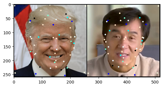
Figure 2.1: Key-points on source (left) and driving (right)

We use a ResNet18² model to predict the key-points. Key-points are just 2D coordinates on an image. So the ResNet outputs a vector with a dimension of K \times N \times 2 and values \in [0,1].

What are those K and N over there??

The model uses multiple deformations (later on that) in this case K is the number of deformation and N is the number of points per deformation. Color

The key-points make no sense, why?

Looking at Figure 2.1 you see that the points appear to be a mess. The reason for the mess is that key-points are trained in a unsupervised manner.

No human interpretable meaning is present while training, what you see right there are locations the model found useful for reconstruction. We can speculate about the structure. For example the points are clustered around the facial outlines, probably because those are the areas that move the most³, but those are speculations.

Infer Optical Flow

Key-points are sparse and lossy representation of what’s going on in the images. We need to use this information to actually estimate how to deform the image to do that we do several things:

Heatmap Representation: Turn sparse key-points into a Gaussian heatmap
Estimate Image Deformation: Key-points represent sparse motion, that is we only know where limited number of points in the source image should move to. To estimate what happens to the other points in the image we learn a Thin-Plate Spline Transformation (TPS).
Occlusion Masks: Image deformation is too simple for the real world (e.g. some parts of the driving image can’t be seen on the source image). We estimate what we don’t know after applying deformation.

Thin-Plate Spline (TPS)

From a birds eye view, TPS takes a 2D points as input and produces 2D point as an output. The idea is to make the TPS tell us where points from the source image should move to match the driving frame. The only known points for us are the key-points we found earlier. We call those the control points of the TPS.

TPSs output for the control points on the driving frame will match the control points on the source frame. Other points will be smoothly moved based on the movement of the control points (weighted by the distance from current points to the control points).

The different colors in Figure 2.1 represent control points for different TPS transforms. Here we will use a bunch of the to deform the image in many different ways. The different TPS transforms are mixed together using weighting coefficients learned by a neural-net

Why do we need occlusion masks?

TPS is a simple transformation compared to the complexity that is required to transform a pose of a person in a real image. Also, TPS is locally accurate, that is only fits the key-points we asked it to fit.

Going outside further from those points we lose accuracy completely. We need to know what are the region we can’t approximate well with a simple image deformation. This can be because a new feature needs to appear (e.g. person shows no teeth in the static image, but needs to show those as part of motion transfer) or because our approximation is bad.

Key Point Normalization

Code

# Detect Key-Points fro the source image and the first frame of the driving video
with th.no_grad():
    kp_src: KPResult
    kp_src = kp_detector(src_img_t)
    kp_drv_init: KPResult
    kp_drv_init = kp_detector(drv_vid_t[:1])


# Load Dense Motion Network
from transmotion.dense_motion import DenseMotionNetwork, DenseMotionResult

dense_motion = DenseMotionNetwork(cfg=conf.dense_motion)
dense_motion = load_orig_weights_to_device(dense_motion)

with th.no_grad():
    kp_src: KPResult
    kp_src = kp_detector(src_img_t)
    kp_drv_init: KPResult
    kp_drv_init = kp_detector(drv_vid_t[:1])


# This functions normalizes source points relative to the change in the driving key-points. 
def dense_infer_normalized_kp(drv_img: th.Tensor) -> DenseMotionResult:
    kp_drv: KPResult
    kp_drv = kp_detector(drv_img.unsqueeze(0))
    kp_norm = kp_src.normalize_relative_to(init_drv=kp_drv_init, cur_drv=kp_drv)
    
    motion_res = dense_motion(
            source_img=src_img_t,
            src_kp=kp_src,
            drv_kp=kp_norm,
            bg_param=None,
            dropout_prob=0.0,
        )
    return motion_res

Inference seems to work better if you only use the change of the driving key-points and not the key points themselves. My guess is that using the change in driving key-points prevents identity information from the driving frame to leak into the source frame (think of Trump’s had getting the shape of the driving video).

What does it mean the change of the driving key-points? We keep initial driving key-points as reference and track the change in the current driving key-points. Next we apply the change in the driving points to the source points, and use the adjusted source as the new driving.

Visualize Dense Motion Results

Code

from transmotion.viz import show_on_gird
from demo_helpers import pils_to_grid, tensors_to_pils, optical_flow_pil 

with th.no_grad():
    res = dense_infer_normalized_kp(drv_vid_t[20])


sparse_deformations = tensors_to_pils(*res.deformed_source[0])

optical_flow = optical_flow_pil(res.optical_flow, size=IMAGE_SIZE)
# Occlusion masks are 1D, we need to turn them into 3D so that they can be on the same grid with everything else
occlusion_masks = [pim.convert("RGB") for pim in tensors_to_pils(*res.occlusion_masks, size=IMAGE_SIZE)]

all_pils = sparse_deformations + [optical_flow] + occlusion_masks
pils_to_grid(*all_pils, size=IMAGE_SIZE)

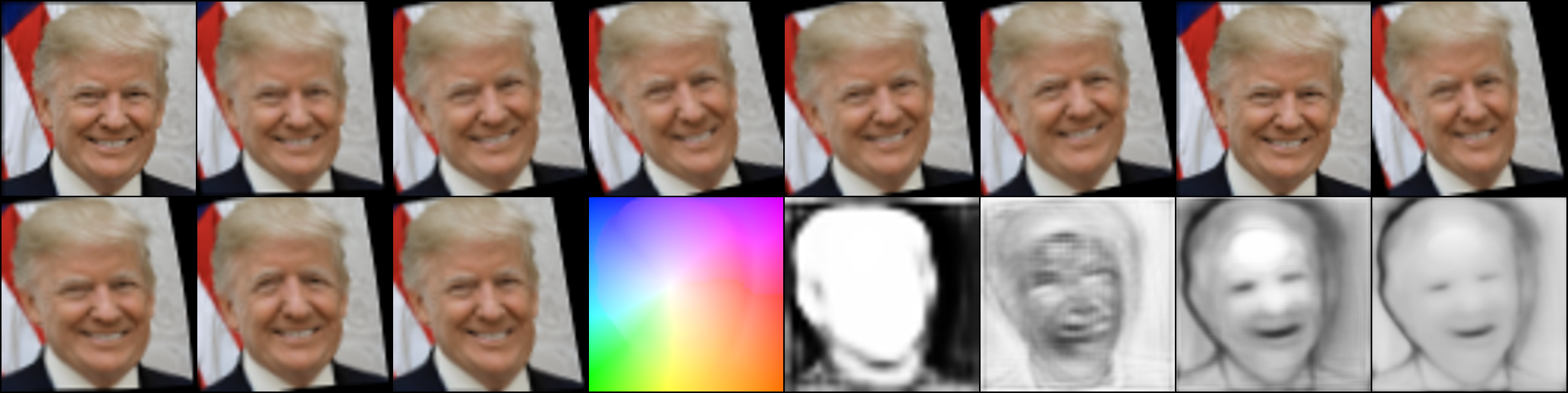
Figure 2.2: TPS Deformed source images, unified optical flow and occlusion masks

in Figure 2.2 the first 11 images (going from left to right) are the deformed source images. The first image represents the backgorund deormations⁴ and the other 10 represent 10 TPS transforms (with 5 control points each). Note that each of the TPSs is pretty simple and kinda looks like a linear transformation. The colorfull image is the resulting optical flow. The last 4 images are the occluiosn masks.⁵

Inpainting the occluded areas

At this point we have the optical flow and the occlusion masks, now its time to inpaint the missing areas from the image. The inpainting is done by an encoder-decoder architecture. We encode the source image and decode back the transformed source image.

The encoding is a series of feature maps on the decoding end, the feature maps get deformed by the optical flow and occluded by the occlusion masks and passed through a decoder layer. So what the encoder-decoder predicts is the occluded areas. At the end of the decoder we take a deformed source image, occlude it and add the predicted occluded areas.

Code

from transmotion.inpainting import InpaintingNetwork, InpaintingResult

inpaint = InpaintingNetwork(cfg=conf.inpainting)
inpaint = load_orig_weights_to_device(inpaint)

inpaint_res: InpaintingResult
inpaint_res = inpaint(
    source_img=src_img_t,
    occlusion_masks=res.occlusion_masks,
    optical_flow=res.optical_flow,
)

from demo_helpers import pil_to_t

broadcaster_occlusion =res.occlusion_masks[-1].repeat(1,3,1,1) 
inv_occlusion = (1 - broadcaster_occlusion)
residual_prediction = (inpaint_res.inpainted_img - inpaint_res.deformed_source*broadcaster_occlusion) / inv_occlusion
occluded_deformed_img = inpaint_res.deformed_source*broadcaster_occlusion

# source, optical flow, deformed
row1 = (src_img_t, pil_to_t(optical_flow).unsqueeze(0), inpaint_res.deformed_source)
# deformed, occlusion, occluded deformed
row2 = (inpaint_res.deformed_source, broadcaster_occlusion, occluded_deformed_img)
# occluded deformed, predicted inpainting, final prediction
row3 = (occluded_deformed_img, residual_prediction, inpaint_res.inpainted_img)

show_on_gird(*(row1+row2+row3), nrow=3)

Figure 2.3: Rows show (1) Optical Flow Deformation (2) Occlusion (3) Inpainting

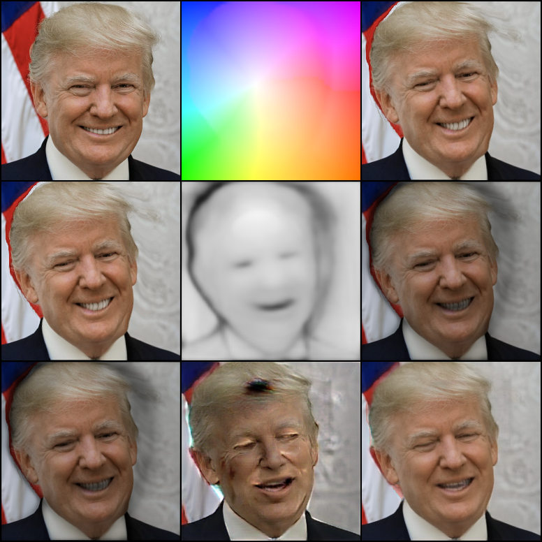
In the rows of Figure 2.3 (going from left to right top to bottom) you can see the original image, the optical flow deformation and the deformed image. Second row starts with the deformed image, show the last occlusion mask and the occluded image. Last row show the occluded image, prediction from the inpainting network and the combination of the two.

Notice

The US flag behind Trump gets deformed (first row on the right). The flag deformation gets occluded (second row on the right) and the final result is Trump occluding the flag and not deformation is visible.

Turning Still Frames to Animation

This part is fairly straight forward, you just do the motion transfer from every driving frame to the source image and turn the transformed sources into a video sequence.

Training Signals

How do we get a training signal for this system? We don’t really have the still image in the pose we want it to get from the driving video. Well the key is to decouple the motion from the identity in the still image.

We represent the driving image as a set of key-points and the motion transfer happens based on those key-points. The driving image used as an input to produce the key-points, as soon as we have those, we don’t need the driving image anymore.

We can train this system as a video reconstruction task. That is, we take the first frame of the driving video and trying to deform it into the next frames of the video. In this case we know how the end result should look like and can train based on this.

Few training source⁶:

we want the output image look the same as the driving image (Perceptual Loss)
we want the key-points to correspond to some interesting features in the image (Equivariance Loss)
The optical flow we learn needs to turn source image to driving image. So we want the deformed source image to have the same encoder feature maps as the driving image. (Optical Flow Loss)

Perceptual Loss

To make sure that the images are the same we use a pre-trained VGG⁷ network and get its feature maps from different scales for both the driving and the source images. Note that we also scale the images.

We put an L_1 loss on the difference between the two sets of feature maps. This loss produces gradients for all the networks in the system.

Equivariance Loss

This loss is to make the key-points correspond to some interesting features. What does that mean? Let’s say we do some known transformation to the image. If the key points correspond to interesting points in the image we expect to see the them transformed in similar fashion. This is exactly what this loss forces the key-points to do. We take an image and its predicted key-points as inputs. Do a random TPS transform on the image and find the key-points of the transformed image. Next we apply the same random TPS transform on the predicted key-points. Finally we put an L_1 loss on the difference between the transformed key-points and the transformed image key-points.

This loss produces gradients for the key-points detection network.

Optical-Flow Loss

The inpainting network has an encoder-decoder architecture. Where the encoder feature maps get deformed and occluded by the optical flow and masks predicted in the dense motion stage. Optical flow is the parts we wish to train. So we want to take the feature maps from the deformed and occluded source image and make them look like the occluded driving image. Once again an L_1 loss is put on the feature differences.

This loss doesn’t train the inpainting encoder nor does it trains the occlusion masks but only for the optical flow.

where each pixel from the source image should move if we want to deform it to match the driving image↩︎
See ResNet Explained by PapersWithCode ↩︎
This particular model was train on the VoX dataset, a dataset of talking faces.↩︎
no deformation in this case.↩︎
Almost everything here was upscaled to 256 \times 256 for visiablilty. Actually most of those are 64 \times 64↩︎
There is additional background transformation loss, that we skip for now.↩︎
VGG exaplained by Papers With Code ↩︎